Markov Chain Fundamentals

A Markov chain is a mathematical system that describes a sequence of events where the probability of each future state depends only on the current state, not on the history of how the system arrived there.

Published: 09/08/2025

A Markov chain is a mathematical system that describes a sequence of events where the probability of each future state depends only on the current state, not on the history of how the system arrived there. This fundamental "memoryless" property, known as the Markov property, makes these stochastic processes essential tools across diverse fields including statistics, economics, genetics, and machine learning.

Transition Matrix Properties

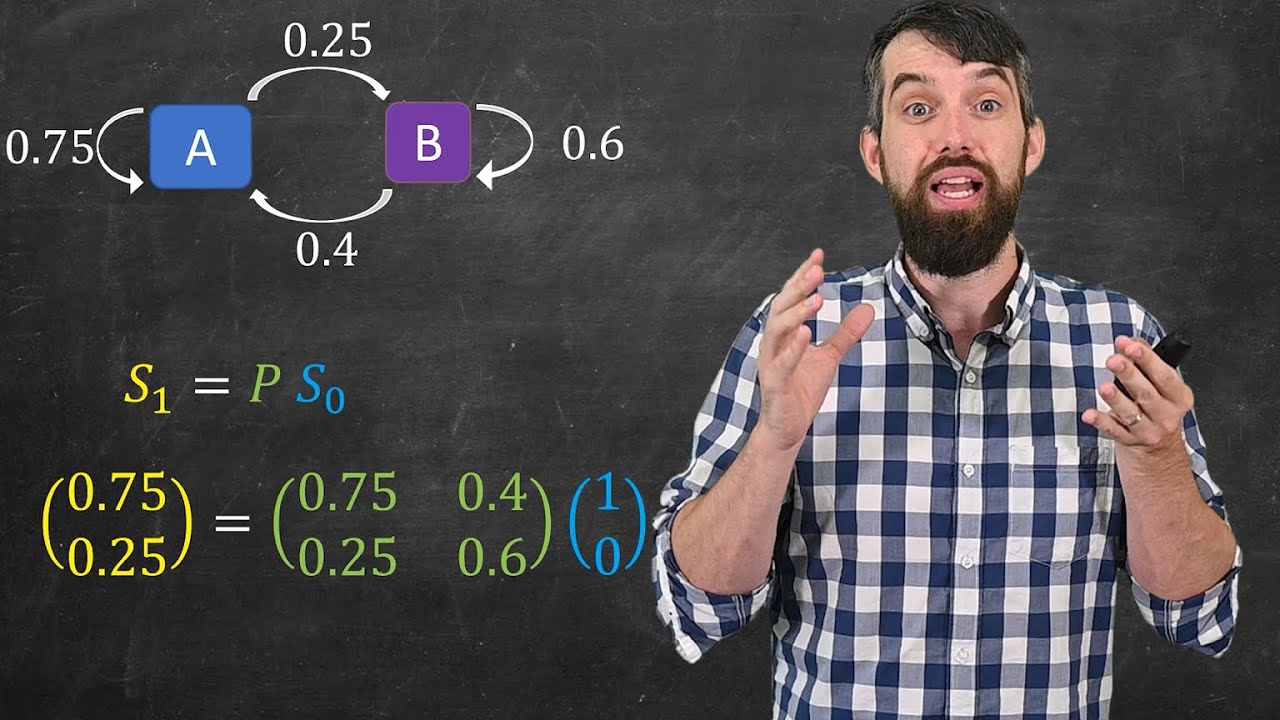
The transition matrix serves as the mathematical backbone of any Markov chain, encoding all possible state transitions as probabilities in a structured format. mit.edu This NxN matrix P organizes transition probabilities $p_{ij}=P(X_{t+1}=j|X_t=i)$ where each element represents the probability of moving from state i to state j. youtube.com The matrix follows specific structural rules that define its behavior: each row must sum to exactly 1, making it a right stochastic matrix, since the probabilities of transitioning from any given state to all possible next states must account for all possibilities. mit.edu

The power of transition matrices lies in their computational efficiency for predicting future states through matrix multiplication. To determine the probability distribution after n steps, one simply computes $P^n$ multiplied by the initial state vector, where $P^n$ represents the transition matrix raised to the nth power. This elegant mathematical framework transforms complex probabilistic calculations into straightforward linear algebra operations, allowing researchers to: youtube.com

• Calculate long-term state probabilities without tracking intermediate steps
• Analyze system behavior through eigenvalues and eigenvectors of the matrix mit.edu
• Identify steady-state distributions and equilibrium conditions ac.nz
• Efficiently model systems with large numbers of possible transitions

Sources: mit.eduyoutube.comyoutube.comac.nzdaniellowengrub.comwikipedia.orgsciencedirect.comnih.govbrilliant.orgsciencedirect.com

Discrete-time Markov chains

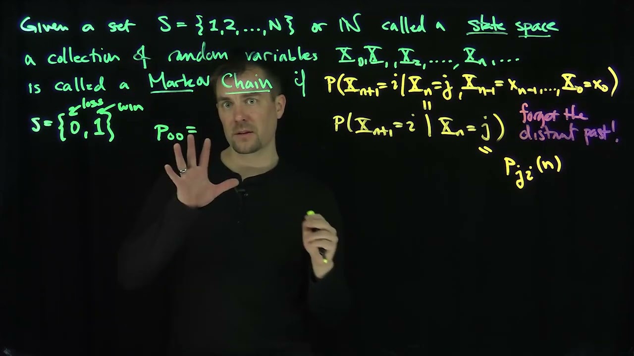
Discrete-time Markov chains operate in distinct time steps, where transitions between states occur at regular intervals denoted as $t=0,1,2,3,...$ This temporal structure creates a sequence of random variables $X_0,X_1,X_2,...$ where each $X_n$ represents the system's state at time n mathworks.com. The defining characteristic emerges in the conditional probability formula: $\text{Pr}(X_{n+1}=x|X_1=x_1,X_2=x_2,...,X_n=x_n)=\text{Pr}(X_{n+1}=x|X_n=x_n)$, provided the conditional probabilities are well-defined mathworks.com.

The discrete-time framework enables precise modeling of systems that change at specific intervals rather than continuously. For instance, a machine alternating between operational state A and error state E might transition with fixed probabilities at each time step: from A to E with 40% probability, remaining in A with 60% probability, while from E it moves to A with 70% probability and stays in E with 30% probability. This temporal discretization proves particularly valuable when analyzing: mathworks.com

• Systems with periodic observations or measurements
• Financial models where state changes occur at market close intervals
• Population genetics where generations represent discrete time steps
• Queue management systems where customers arrive at regular intervals wikipedia.org

The state space can range from finite sets for simple binary systems to countable infinite sets for more complex scenarios, with the discrete-time structure maintaining mathematical tractability through matrix operations and iterative calculations. washington.educolumbia.edu

Sources: mathworks.comwikipedia.orgwashington.educolumbia.eduac.ukprobabilitycourse.comac.uktimeseriesreasoning.comyoutube.com

Continuous-time Markov chains

Continuous-time Markov chains (CTMCs) extend the Markov framework to scenarios where state transitions can occur at any moment rather than fixed intervals, making them ideal for modeling real-world systems that evolve continuously. Unlike their discrete-time counterparts, CTMCs are governed by rate matrices (also called generator matrices or intensity matrices) denoted as Q, where each element $q_{ij}$ represents the instantaneous rate of transitioning from state i to state j. The diagonal elements $q_{ii}$ are negative and equal to $-{\sum }_{j\ne i}{q}_{ij}$, ensuring that each row sums to zero—a fundamental property distinguishing rate matrices from probability matrices. jair.orgwikipedia.org

The continuous-time structure introduces exponential waiting times between transitions, where the time spent in any state follows an exponential distribution with parameter equal to the negative diagonal element of that state's row. This memoryless property of exponential distributions preserves the Markov characteristic in continuous time. Key applications demonstrate the versatility of CTMCs: jair.org

• Biological modeling: DNA evolution models where nucleotide substitutions occur at continuous rates over evolutionary time mit.edu
• Reliability engineering: Systems where component failures happen randomly in continuous time
• Queueing theory: Service systems where arrivals and departures occur at varying continuous rates
• Chemical kinetics: Reaction networks where molecular interactions follow continuous stochastic processes

The mathematical analysis of CTMCs often employs uniformization techniques, which convert continuous-time problems into discrete-time equivalents by constructing a stochastic matrix $M=Q/\alpha +I$ where $\alpha$ exceeds the maximum rate in the system. This approach enables researchers to leverage discrete-time computational methods while maintaining the continuous-time model's accuracy and interpretability. wikipedia.org

Sources: jair.orgwikipedia.orgmit.educolumbia.edutsourakakis.comalooba.comjaro.inarxiv.org